Gradient descent
梯度下降。
Gradient descent
Gradient descent is a first-order iterative optimization algorithm for finding the minimum of a function. To find a local minimum of a function using gradient descent, one takes steps proportional to the negative of the gradient (or approximate gradient) of the function at the current point. If, instead, one takes steps proportional to the positive of the gradient, one approaches a local maximum of that function; the procedure is then known as gradient ascent.
SUMMARY : 梯度上升与梯度下降
Gradient descent is also known as steepest descent(极速下降). However, gradient descent should not be confused with the method of steepest descent for approximating integrals.
Description
Gradient descent is based on the observation that if the multi-variable function $ F(\mathbf {x} ) $ is defined and differentiable in a neighborhood of a point $ \mathbf {a} $, then $ F(\mathbf {x} ) $ decreases fastest if one goes from $ \mathbf {a} $ in the direction of the negative gradient of $ F $ at $ \mathbf {a} ,-\nabla F(\mathbf {a} ) $. It follows that, if
$ \mathbf {a} _{n+1}=\mathbf {a} _{n}-\gamma \nabla F(\mathbf {a} _{n}) $
for $ \gamma \in \mathbb {R} {+} $ small enough, then $ F(\mathbf {a{n}} )\geq F(\mathbf {a_{n+1}} ) $. In other words, the term $ \gamma \nabla F(\mathbf {a} ) $ is subtracted from $ \mathbf {a} $ because we want to move against the gradient, toward the minimum. With this observation in mind, one starts with a guess $ \mathbf {x} _{0} $ for a local minimum of $ F $, and considers the sequence $ \mathbf {x} _{0},\mathbf {x} _{1},\mathbf {x} _{2},\ldots $ such that
$ \mathbf {x} _{n+1}=\mathbf {x} _{n}-\gamma _{n}\nabla F(\mathbf {x} _{n}), n\geq 0. $
We have a monotonic sequence
$ F(\mathbf {x} _{0})\geq F(\mathbf {x} _{1})\geq F(\mathbf {x} _{2})\geq \cdots , $
so hopefully the sequence $ (\mathbf {x} _{n}) $ converges to the desired local minimum. Note that the value of the step size $ \gamma $ is allowed to change at every iteration. With certain assumptions on the function $ F $ (for example, $ F $ convex and $ \nabla F $ Lipschitz) and particular choices of $ \gamma $ (e.g., chosen either via a line search that satisfies the Wolfe conditions or the Barzilai-Borwein[1] method shown as following),
$ \gamma _{n}={\frac {\left|\left(\mathbf {x} _{n}-\mathbf {x} _{n-1}\right)^{T}\left[\nabla F(\mathbf {x} _{n})-\nabla F(\mathbf {x} _{n-1})\right]\right|}{\left|\nabla F(\mathbf {x} _{n})-\nabla F(\mathbf {x} _{n-1})\right|^{2}}} $
convergence to a local minimum can be guaranteed. When the function $ F $ is convex, all local minima are also global minima, so in this case gradient descent can converge to the global solution.
This process is illustrated in the adjacent picture. Here $ F $ is assumed to be defined on the plane, and that its graph has a bowl shape. The blue curves are the contour lines, that is, the regions on which the value of $ F $ is constant. A red arrow originating at a point shows the direction of the negative gradient at that point. Note that the (negative) gradient at a point is orthogonal to the contour line going through that point. We see that gradient descent leads us to the bottom of the bowl, that is, to the point where the value of the function $ F $ is minimal.
 Illustration of gradient descent on a series of level sets.
Examples
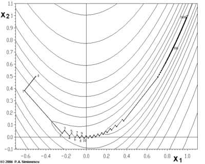
Gradient descent has problems with pathological(病态) functions such as the Rosenbrock function shown here.
$ f(x_{1},x_{2})=(1-x_{1}){2}+100(x_{2}-{x_{1}}{2})^{2}. $
The Rosenbrock function has a narrow curved valley which contains the minimum. The bottom of the valley is very flat. Because of the curved flat valley the optimization is zigzagging slowly with small step sizes towards the minimum.
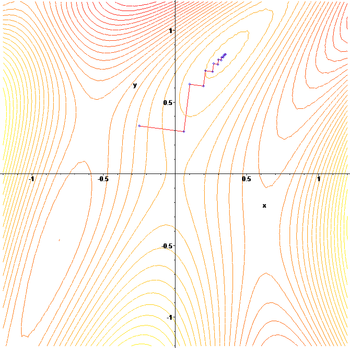
The zigzagging nature of the method is also evident below, where the gradient descent method is applied to
$ F(x,y)=\sin \left({\frac {1}{2}}x^{2}-{\frac {1}{4}}y^{2}+3\right)\cos \left(2x+1-e^{y}\right). $


