Convolutional Neural Networks (CNNs / ConvNets)

Convolutional Neural Networks are very similar to ordinary Neural Networks from the previous chapter: they are made up of neurons that have learnable weights and biases. Each neuron receives some inputs, performs a dot product and optionally follows it with a non-linearity. The whole network still expresses a single differentiable score function: from the raw image pixels on one end to class scores at the other. And they still have a loss function (e.g. SVM/Softmax) on the last (fully-connected) layer and all the tips/tricks we developed for learning regular Neural Networks still apply.

SUMMARY : dot product意味着结果是一个张量；意味着filter的shape和它所扫过的区域的shape相同；

SUMMARY : score function vs loss function

SUMMARY : The whole network still expresses a single differentiable score function

So what changes? ConvNet architectures make the explicit assumption that the inputs are images, which allows us to encode certain properties into the architecture. These then make the forward function more efficient to implement and vastly reduce the amount of parameters in the network.

Architecture Overview

Recall: Regular Neural Nets. As we saw in the previous chapter, Neural Networks receive an input (a single vector), and transform it through a series of hidden layers. Each hidden layer is made up of a set of neurons, where each neuron is fully connected to all neurons in the previous layer, and where neurons in a single layer function completely independently and do not share any connections. The last fully-connected layer is called the “output layer” and in classification settings it represents the class scores.

Regular Neural Nets don’t scale well to full images. In CIFAR-10, images are only of size 32x32x3 (32 wide, 32 high, 3 color channels), so a single fully-connected neuron in a first hidden layer of a regular Neural Network would have $32*32*3 = 3072$ weights. This amount still seems manageable, but clearly this fully-connected structure does not scale to larger images. For example, an image of more respectable size, e.g. $200 * 200 * 3$, would lead to neurons that have $200*200*3 = 120,000$ weights. Moreover, we would almost certainly want to have several such neurons, so the parameters would add up quickly! Clearly, this full connectivity is wasteful and the huge number of parameters would quickly lead to overfitting.

3D volumes of neurons. Convolutional Neural Networks take advantage of the fact that the input consists of images and they constrain the architecture in a more sensible way. In particular, unlike a regular Neural Network, the layers of a ConvNet have neurons arranged in 3 dimensions: width, height, depth. (Note that the word depth here refers to the third dimension of an activation volume, not to the depth of a full Neural Network, which can refer to the total number of layers in a network.) For example, the input images in CIFAR-10 are an input volume of activations, and the volume has dimensions 32x32x3​ (width, height, depth respectively). As we will soon see, the neurons in a layer will only be connected to a small region of the layer before it, instead of all of the neurons in a fully-connected manner. Moreover, the final output layer would for CIFAR-10 have dimensions 1x1x10​, because by the end of the ConvNet architecture we will reduce the full image into a single vector of class scores, arranged along the depth dimension. Here is a visualization:

---

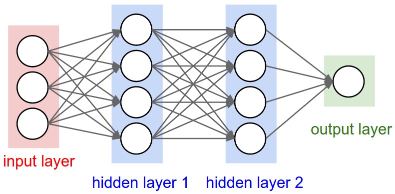
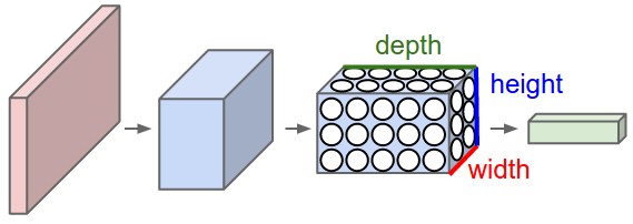
Left: A regular 3-layer Neural Network. Right: A ConvNet arranges its neurons in three dimensions (width, height, depth), as visualized in one of the layers. Every layer of a ConvNet transforms the 3D input volume to a 3D output volume of neuron activations. In this example, the red input layer holds the image, so its width and height would be the dimensions of the image, and the depth would be 3 (Red, Green, Blue channels).

---

A ConvNet is made up of Layers. Every Layer has a simple API: It transforms an input 3D volume to an output 3D volume with some differentiable function that may or may not have parameters.

Layers used to build ConvNets

As we described above, a simple ConvNet is a sequence of layers, and every layer of a ConvNet transforms one volume of activations to another through a differentiable function. We use three main types of layers to build ConvNet architectures: Convolutional Layer, Pooling Layer, and Fully-Connected Layer (exactly as seen in regular Neural Networks). We will stack these layers to form a full ConvNet architecture.

Example Architecture: Overview. We will go into more details below, but a simple ConvNet for CIFAR-10 classification could have the architecture [INPUT - CONV - RELU - POOL - FC]. In more detail:

• INPUT [32x32x3] will hold the raw pixel values of the image, in this case an image of width 32, height 32, and with three color channels R,G,B.
• CONV layer will compute the output of neurons that are connected to local regions in the input, each computing a dot product between their weights and a small region they are connected to in the input volume. This may result in volume such as [32x32x12] if we decided to use 12 filters.
• RELU layer will apply an elementwise activation function, such as the $max(0,x)$ thresholding at zero. This leaves the size of the volume unchanged ([32x32x12]).
• POOL layer will perform a downsampling operation along the spatial dimensions (width, height), resulting in volume such as [16x16x12].
• FC (i.e. fully-connected) layer will compute the class scores, resulting in volume of size [1x1x10], where each of the 10 numbers correspond to a class score, such as among the 10 categories of CIFAR-10. As with ordinary Neural Networks and as the name implies, each neuron in this layer will be connected to all the numbers in the previous volume.

In this way, ConvNets transform the original image layer by layer from the original pixel values to the final class scores. Note that some layers contain parameters and other don’t. In particular, the CONV/FC layers perform transformations that are a function of not only the activations in the input volume, but also of the parameters (the weights and biases of the neurons). On the other hand, the RELU/POOL layers will implement a fixed function. The parameters in the CONV/FC layers will be trained with gradient descent so that the class scores that the ConvNet computes are consistent with the labels in the training set for each image.

In summary:

• A ConvNet architecture is in the simplest case a list of Layers that transform the image volume into an output volume (e.g. holding the class scores)
• There are a few distinct types of Layers (e.g. CONV/FC/RELU/POOL are by far the most popular)
• Each Layer accepts an input 3D volume and transforms it to an output 3D volume through a differentiable function
• Each Layer may or may not have parameters (e.g. CONV/FC do, RELU/POOL don’t)
• Each Layer may or may not have additional hyperparameters (e.g. CONV/FC/POOL do, RELU doesn’t)

---

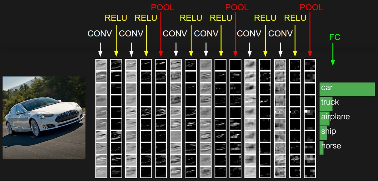The activations of an example ConvNet architecture. The initial volume stores the raw image pixels (left) and the last volume stores the class scores (right). Each volume of activations along the processing path is shown as a column. Since it's difficult to visualize 3D volumes, we lay out each volume's slices in rows. The last layer volume holds the scores for each class, but here we only visualize the sorted top 5 scores, and print the labels of each one. The full web-based demo is shown in the header of our website. The architecture shown here is a tiny VGG Net, which we will discuss later.

---

We now describe the individual layers and the details of their hyperparameters and their connectivities.

Convolutional Layer

The Conv layer is the core building block of a Convolutional Network that does most of the computational heavy lifting.

Conv层是卷积网络的核心构件，它承担了大部分计算量。

SUMMARY : 下面几段，从不同的角度对CNN进行了描述，**Overview and intuition without brain stuff**段是从数学（卷积运算）的角度进行的描述，**The brain view**段则是从neuron的角度来进行的描述；其实从这个角度来看，我们所使用的network topology其实是对数学运算的形象化：MLP中所谓的全连接，其实是对矩阵乘法的形象化；CNN中的情况在下面给出了非常详细的介绍；那这两者到底是先有的数学，然后有的对它的形象化的描述呢？还是先有的后者再有的前者？

Overview and intuition without brain stuff.

Lets first discuss what the CONV layer computes without brain/neuron analogies. The CONV layer’s parameters consist of a set of learnable filters. Every filter is small spatially (along width and height), but extends through the full depth of the input volume. For example, a typical filter on a first layer of a ConvNet might have size 5x5x3 (i.e. 5 pixels width and height, and 3 because images have depth 3, the color channels). During the forward pass, we slide（滑动） (more precisely, convolve（卷积）) each filter across the width and height of the input volume and compute dot products between the entries of the filter and the input at any position. As we slide the filter over the width and height of the input volume we will produce a 2-dimensional activation map that gives the responses of that filter at every spatial position. Intuitively, the network will learn filters that activate when they see some type of visual feature such as an edge（边缘） of some orientation or a blotch（斑点） of some color on the first layer, or eventually entire honeycomb or wheel-like patterns on higher layers of the network. Now, we will have an entire set of filters in each CONV layer (e.g. 12 filters), and each of them will produce a separate 2-dimensional activation map. We will stack these activation maps along the depth dimension and produce the output volume.

没有大脑的概述和直觉。让我们首先讨论CONV层在没有脑/神经元类比的情况下计算的内容。 CONV层的参数由一组可学习的过滤器组成。每个过滤器在空间上都很小（沿宽度和高度），但延伸到输入体积的整个深度。例如，ConvNet第一层上的典型滤波器可能具有5x5x3的尺寸（即5像素宽度和高度，以及3，因为图像具有深度3，颜色通道）。在前向传递期间，我们在输入体积的宽度和高度上滑动（滑动）（更准确地说，卷积（卷积））每个滤波器，并计算滤波器的条目和任何位置处的输入之间的点积。当我们在输入体积的宽度和高度上滑动滤镜时，我们将生成一个二维激活贴图，该贴图在每个空间位置给出该滤镜的响应。直观地，网络将学习当他们看到某种类型的视觉特征时激活的过滤器，例如某个方向的边缘或第一层上某种颜色的斑点，或最终在网络的更高层上的整个蜂窝或轮状图案。现在，我们将在每个CONV层中有一整套过滤器（例如12个过滤器），并且每个过滤器将产生单独的2维激活图。我们将沿深度维度堆叠这些激活图并生成输出量。

THINKING : 每个filter是否需要扫描完整个**input volume**？每个filter的输出是什么？ entries of the filter的含义是什么？这些问题在上面这一段中都已经描述清楚了；

THINKING : 所谓的filter，其实就是一个卷积运算子；

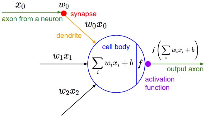
The brain view.

If you’re a fan of the brain/neuron analogies, every entry in the 3D output volume can also be interpreted as an output of a neuron that looks at only a small region in the input and shares parameters with all neurons to the left and right spatially (since these numbers all result from applying the same filter). We now discuss the details of the neuron connectivities, their arrangement in space, and their parameter sharing scheme.

THINKING : neuron和filter之间的关系？？按照MLP中的理解，每一层中的一个neuron都执行了一个function，那在CNN中，是否也是如此呢？在下面这一段中就会介绍这个内容，其实通过这个内容也可以得知：在CNN中，每个neuron所执行的都是一个filter的操作；

Local Connectivity.

When dealing with high-dimensional inputs such as images, as we saw above it is impractical to connect neurons to all neurons in the previous volume. Instead, we will connect each neuron to only a local region of the input volume. The spatial extent of this connectivity is a hyperparameter called the receptive field of the neuron (equivalently（相当于） this is the filter size). The extent of the connectivity along the depth axis is always equal to the depth of the input volume. It is important to emphasize again this asymmetry in how we treat the spatial dimensions (width and height) and the depth dimension: The connections are local in space (along width and height), but always full along the entire depth of the input volume.

Example 1. For example, suppose that the input volume has size [32x32x3], (e.g. an RGB CIFAR-10 image). If the receptive field (or the filter size) is 5x5, then each neuron in the Conv Layer will have weights to a [5x5x3] region in the input volume, for a total of $5*5*3 = 75$ weights (and +1 bias parameter). Notice that the extent of the connectivity along the depth axis must be 3, since this is the depth of the input volume.

Example 2. Suppose an input volume had size [16x16x20]. Then using an example receptive field size of 3x3, every neuron in the Conv Layer would now have a total of $3*3*20 = 180$ connections to the input volume. Notice that, again, the connectivity is local in space (e.g. 3x3), but full along the input depth (20).

---

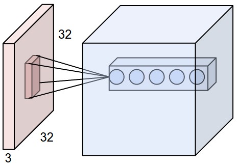
Left: An example input volume in red (e.g. a 32x32x3 CIFAR-10 image), and an example volume of neurons in the first Convolutional layer. Each neuron in the convolutional layer is connected only to a local region in the input volume spatially, but to the full depth (i.e. all color channels). Note, there are multiple neurons (5 in this example) along the depth, all looking at the same region in the input - see discussion of depth columns in text below. Right: The neurons from the Neural Network chapter remain unchanged: They still compute a dot product of their weights with the input followed by a non-linearity, but their connectivity is now restricted to be local spatially.

---

Spatial arrangement.

We have explained the connectivity of each neuron in the Conv Layer to the input volume, but we haven’t yet discussed how many neurons there are in the output volume or how they are arranged. Three hyperparameters control the size of the output volume: the depth, stride and zero-padding. We discuss these next:

1. First, the depth of the output volume is a hyperparameter: it corresponds to the number of filters we would like to use, each learning to look for something different in the input. For example, if the first Convolutional Layer takes as input the raw image, then different neurons along the depth dimension may activate in presence of various oriented edges, or blobs of color. We will refer to a set of neurons that are all looking at the same region of the input as a depth column (some people also prefer the term fibre).
2. Second, we must specify the stride with which we slide the filter. When the stride is 1 then we move the filters one pixel at a time. When the stride is 2 (or uncommonly 3 or more, though this is rare in practice) then the filters jump 2 pixels at a time as we slide them around. This will produce smaller output volumes spatially.
3. As we will soon see, sometimes it will be convenient to pad the input volume with zeros around the border. The size of this zero-padding is a hyperparameter. The nice feature of zero padding is that it will allow us to control the spatial size of the output volumes (most commonly as we’ll see soon we will use it to exactly preserve the spatial size of the input volume so the input and output width and height are the same).

We can compute the spatial size of the output volume as a function of the input volume size ($W$), the receptive field size of the Conv Layer neurons ($F$), the stride with which they are applied ($S$), and the amount of zero padding used ($P$) on the border. You can convince yourself that the correct formula for calculating how many neurons “fit” is given by $(W - F + 2P)/S + 1$. For example for a 7x7 input and a 3x3 filter with stride 1 and pad 0 we would get a 5x5 output. With stride 2 we would get a 3x3 output. Lets also see one more graphical example:

---

Illustration of spatial arrangement. In this example there is only one spatial dimension (x-axis), one neuron with a receptive field size of F = 3, the input size is W = 5, and there is zero padding of P = 1. Left: The neuron strided across the input in stride of S = 1, giving output of size (5 - 3 + 2)/1+1 = 5. Right: The neuron uses stride of S = 2, giving output of size (5 - 3 + 2)/2+1 = 3. Notice that stride S = 3 could not be used since it wouldn't fit neatly across the volume. In terms of the equation, this can be determined since (5 - 3 + 2) = 4 is not divisible by 3. The neuron weights are in this example [1,0,-1] (shown on very right), and its bias is zero. These weights are shared across all yellow neurons (see parameter sharing below).

---

Use of zero-padding. In the example above on left, note that the input dimension was 5 and the output dimension was equal: also 5. This worked out so because our receptive fields were 3 and we used zero padding of 1. If there was no zero-padding used, then the output volume would have had spatial dimension of only 3, because that it is how many neurons would have “fit” across the original input. In general, setting zero padding to be $P=(F−1)/2$ when the stride is $S=1$ ensures that the input volume and output volume will have the same size spatially. It is very common to use zero-padding in this way and we will discuss the full reasons when we talk more about ConvNet architectures.

Constraints on strides. Note again that the spatial arrangement hyperparameters have mutual constraints. For example, when the input has size $W=10$, no zero-padding is used $P=0$, and the filter size is $F=3$, then it would be impossible to use stride $S=2$, since , i.e. not an integer, indicating that the neurons don’t “fit” neatly and symmetrically across the input. Therefore, this setting of the hyperparameters is considered to be invalid, and a ConvNet library could throw an exception or zero pad the rest to make it fit, or crop the input to make it fit, or something. As we will see in the ConvNet architectures section, sizing the ConvNets appropriately so that all the dimensions “work out” can be a real headache, which the use of zero-padding and some design guidelines will significantly alleviate.

Real-world example. The Krizhevsky et al. architecture that won the ImageNet challenge in 2012 accepted images of size [227x227x3]. On the first Convolutional Layer, it used neurons with receptive field size $F=11$, stride $S=4$ and no zero padding $P=0$. Since (227 - 11)/4 + 1 = 55, and since the Conv layer had a depth of $K=96$, the Conv layer output volume had size [55x55x96]. Each of the 55*55*96 neurons in this volume was connected to a region of size [11x11x3] in the input volume. Moreover, all 96 neurons in each depth column are connected to the same [11x11x3] region of the input, but of course with different weights. As a fun aside, if you read the actual paper it claims that the input images were 224x224, which is surely incorrect because (224 - 11)/4 + 1 is quite clearly not an integer. This has confused many people in the history of ConvNets and little is known about what happened. My own best guess is that Alex used zero-padding of 3 extra pixels that he does not mention in the paper.

Parameter Sharing.

Parameter sharing scheme is used in Convolutional Layers to control the number of parameters. Using the real-world example above, we see that there are 55*55*96 = 290,400 neurons in the first Conv Layer, and each has 11*11*3 = 363 weights and 1 bias. Together, this adds up to 290400 * 364 = 105,705,600 parameters on the first layer of the ConvNet alone. Clearly, this number is very high.

It turns out that we can dramatically reduce the number of parameters by making one reasonable assumption: That if one feature is useful to compute at some spatial position (x,y), then it should also be useful to compute at a different position (x2,y2). In other words, denoting a single 2-dimensional slice of depth as a depth slice (e.g. a volume of size [55x55x96] has 96 depth slices, each of size [55x55]), we are going to constrain the neurons in each depth slice to use the same weights and bias. With this parameter sharing scheme, the first Conv Layer in our example would now have only 96 unique set of weights (one for each depth slice), for a total of 96*11*11*3 = 34,848 unique weights, or 34,944 parameters (+96 biases). Alternatively, all 55*55 neurons in each depth slice will now be using the same parameters. In practice during backpropagation, every neuron in the volume will compute the gradient for its weights, but these gradients will be added up across each depth slice and only update a single set of weights per slice.

Notice that if all neurons in a single depth slice are using the same weight vector, then the forward pass of the CONV layer can in each depth slice be computed as a convolution of the neuron’s weights with the input volume (Hence the name: Convolutional Layer). This is why it is common to refer to the sets of weights as a filter (or a kernel), that is convolved with the input.

---

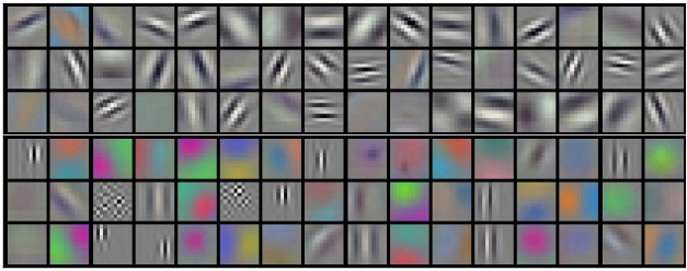Example filters learned by Krizhevsky et al. Each of the 96 filters shown here is of size [11x11x3], and each one is shared by the 55*55 neurons in one depth slice. Notice that the parameter sharing assumption is relatively reasonable: If detecting a horizontal edge is important at some location in the image, it should intuitively be useful at some other location as well due to the translationally-invariant structure of images. There is therefore no need to relearn to detect a horizontal edge at every one of the 55*55 distinct locations in the Conv layer output volume.

---

Note that sometimes the parameter sharing assumption may not make sense. This is especially the case when the input images to a ConvNet have some specific centered structure, where we should expect, for example, that completely different features should be learned on one side of the image than another. One practical example is when the input are faces that have been centered in the image. You might expect that different eye-specific or hair-specific features could (and should) be learned in different spatial locations. In that case it is common to relax the parameter sharing scheme, and instead simply call the layer a Locally-Connected Layer.

Numpy examples.

To make the discussion above more concrete, lets express the same ideas but in code and with a specific example. Suppose that the input volume is a numpy array X. Then:

• A depth column (or a fibre) at position (x,y) would be the activations X[x,y,:].
• A depth slice, or equivalently an activation map at depth d would be the activations X[:,:,d].

Conv Layer Example. Suppose that the input volume X has shape X.shape: (11,11,4). Suppose further that we use no zero padding (P=0P=0), that the filter size is F=5F=5, and that the stride is S=2S=2. The output volume would therefore have spatial size (11-5)/2+1 = 4, giving a volume with width and height of 4. The activation map in the output volume (call it V), would then look as follows (only some of the elements are computed in this example):

• V[0,0,0] = np.sum(X[:5,:5,:] * W0) + b0
• V[1,0,0] = np.sum(X[2:7,:5,:] * W0) + b0
• V[2,0,0] = np.sum(X[4:9,:5,:] * W0) + b0
• V[3,0,0] = np.sum(X[6:11,:5,:] * W0) + b0

Remember that in numpy, the operation * above denotes elementwise multiplication between the arrays. Notice also that the weight vector W0 is the weight vector of that neuron and b0 is the bias. Here, W0 is assumed to be of shape W0.shape: (5,5,4), since the filter size is 5 and the depth of the input volume is 4. Notice that at each point, we are computing the dot product as seen before in ordinary neural networks. Also, we see that we are using the same weight and bias (due to parameter sharing), and where the dimensions along the width are increasing in steps of 2 (i.e. the stride). To construct a second activation map in the output volume, we would have:

• V[0,0,1] = np.sum(X[:5,:5,:] * W1) + b1
• V[1,0,1] = np.sum(X[2:7,:5,:] * W1) + b1
• V[2,0,1] = np.sum(X[4:9,:5,:] * W1) + b1
• V[3,0,1] = np.sum(X[6:11,:5,:] * W1) + b1
• V[0,1,1] = np.sum(X[:5,2:7,:] * W1) + b1 (example of going along y)
• V[2,3,1] = np.sum(X[4:9,6:11,:] * W1) + b1 (or along both)

where we see that we are indexing into the second depth dimension in V (at index 1) because we are computing the second activation map, and that a different set of parameters (W1) is now used. In the example above, we are for brevity leaving out some of the other operations the Conv Layer would perform to fill the other parts of the output array V. Additionally, recall that these activation maps are often followed elementwise through an activation function such as ReLU, but this is not shown here.

Summary. To summarize, the Conv Layer:

• Accepts a volume of size W1×H1×D1W1×H1×D1

• Requires four hyperparameters:

• Number of filters KK,

• their spatial extent FF,
• the stride SS,

• the amount of zero padding PP.

• Produces a volume of size

W2×H2×D2W2×H2×D2

where:

• W2=(W1−F+2P)/S+1W2=(W1−F+2P)/S+1
• H2=(H1−F+2P)/S+1H2=(H1−F+2P)/S+1 (i.e. width and height are computed equally by symmetry)

• D2=KD2=K

• With parameter sharing, it introduces F⋅F⋅D1F⋅F⋅D1 weights per filter, for a total of (F⋅F⋅D1)⋅K(F⋅F⋅D1)⋅K weights and KK biases.

• In the output volume, the dd-th depth slice (of size W2×H2W2×H2) is the result of performing a valid convolution of the dd-th filter over the input volume with a stride of SS, and then offset by dd-th bias.

A common setting of the hyperparameters is F=3,S=1,P=1F=3,S=1,P=1. However, there are common conventions and rules of thumb that motivate these hyperparameters. See the ConvNet architectures section below.

Convolution Demo.

Below is a running demo of a CONV layer. Since 3D volumes are hard to visualize, all the volumes (the input volume (in blue), the weight volumes (in red), the output volume (in green)) are visualized with each depth slice stacked in rows. The input volume is of size $W_1 = 5, H_1 = 5, D_1 = 3$, and the CONV layer parameters are $K = 2, F = 3, S = 2, P = 1$. That is, we have two filters of size 3×33×3, and they are applied with a stride of 2. Therefore, the output volume size has spatial size (5 - 3 + 2)/2 + 1 = 3. Moreover, notice that a padding of $P=1$ is applied to the input volume, making the outer border of the input volume zero. The visualization below iterates over the output activations (green), and shows that each element is computed by elementwise multiplying the highlighted input (blue) with the filter (red), summing it up, and then offsetting the result by the bias.

---

---

Implementation as Matrix Multiplication.

Note that the convolution operation essentially performs dot products between the filters and local regions of the input. A common implementation pattern of the CONV layer is to take advantage of this fact and formulate the forward pass of a convolutional layer as one big matrix multiply as follows:

1. The local regions in the input image are stretched out into columns in an operation commonly called im2col. For example, if the input is [227x227x3] and it is to be convolved with 11x11x3 filters at stride 4, then we would take [11x11x3] blocks of pixels in the input and stretch each block into a column vector of size 11*11*3 = 363. Iterating this process in the input at stride of 4 gives (227-11)/4+1 = 55 locations along both width and height, leading to an output matrix X_col of im2col of size [363 x 3025], where every column is a stretched out receptive field and there are 55*55 = 3025 of them in total. Note that since the receptive fields overlap, every number in the input volume may be duplicated in multiple distinct columns.
2. The weights of the CONV layer are similarly stretched out into rows. For example, if there are 96 filters of size [11x11x3] this would give a matrix W_row of size [96 x 363].
3. The result of a convolution is now equivalent to performing one large matrix multiply np.dot(W_row, X_col), which evaluates the dot product between every filter and every receptive field location. In our example, the output of this operation would be [96 x 3025], giving the output of the dot product of each filter at each location.
4. The result must finally be reshaped back to its proper output dimension [55x55x96].

This approach has the downside that it can use a lot of memory, since some values in the input volume are replicated multiple times in X_col. However, the benefit is that there are many very efficient implementations of Matrix Multiplication that we can take advantage of (for example, in the commonly used BLAS API). Moreover, the same im2col idea can be reused to perform the pooling operation, which we discuss next.

Backpropagation.

The backward pass for a convolution operation (for both the data and the weights) is also a convolution (but with spatially-flipped filters). This is easy to derive in the 1-dimensional case with a toy example (not expanded on for now).

1x1 convolution.

As an aside, several papers use 1x1 convolutions, as first investigated by Network in Network. Some people are at first confused to see 1x1 convolutions especially when they come from signal processing background. Normally signals are 2-dimensional so 1x1 convolutions do not make sense (it’s just pointwise scaling). However, in ConvNets this is not the case because one must remember that we operate over 3-dimensional volumes, and that the filters always extend through the full depth of the input volume. For example, if the input is [32x32x3] then doing 1x1 convolutions would effectively be doing 3-dimensional dot products (since the input depth is 3 channels).

Dilated convolutions.

A recent development (e.g. see paper by Fisher Yu and Vladlen Koltun) is to introduce one more hyperparameter to the CONV layer called the dilation. So far we’ve only discussed CONV filters that are contiguous. However, it’s possible to have filters that have spaces between each cell, called dilation. As an example, in one dimension a filter w of size 3 would compute over input x the following: w[0]*x[0] + w[1]*x[1] + w[2]*x[2]. This is dilation of 0. For dilation 1 the filter would instead compute w[0]*x[0] + w[1]*x[2] + w[2]*x[4]; In other words there is a gap of 1 between the applications. This can be very useful in some settings to use in conjunction with 0-dilated filters because it allows you to merge spatial information across the inputs much more agressively with fewer layers. For example, if you stack two 3x3 CONV layers on top of each other then you can convince yourself that the neurons on the 2^nd layer are a function of a 5x5 patch of the input (we would say that the effective receptive field of these neurons is 5x5). If we use dilated convolutions then this effective receptive field would grow much quicker.

Pooling Layer

It is common to periodically insert a Pooling layer in-between successive Conv layers in a ConvNet architecture. Its function is to progressively reduce the spatial size of the representation to reduce the amount of parameters and computation in the network, and hence to also control overfitting. The Pooling Layer operates independently on every depth slice of the input and resizes it spatially, using the MAX operation. The most common form is a pooling layer with filters of size 2x2 applied with a stride of 2 downsamples every depth slice in the input by 2 along both width and height, discarding 75% of the activations. Every MAX operation would in this case be taking a max over 4 numbers (little 2x2 region in some depth slice). The depth dimension remains unchanged. More generally, the pooling layer:

• Accepts a volume of size $W_1 \times H_1 \times D_1$
• Requires two hyperparameters:
• their spatial extent $F$,
• the stride $S$,
• Produces a volume of size $W_2 \times H_2 \times D_2$ where:
• $W_2 = (W_1 - F)/S + 1$
• $H_2 = (H_1 - F)/S + 1$
• $D_2 = D_1$
• Introduces zero parameters since it computes a fixed function of the input
• For Pooling layers, it is not common to pad the input using zero-padding.

It is worth noting that there are only two commonly seen variations of the max pooling layer found in practice: A pooling layer with $F=3,S=2$ (also called overlapping pooling), and more commonly $F=2,S=2$. Pooling sizes with larger receptive fields are too destructive.

General pooling.

In addition to max pooling, the pooling units can also perform other functions, such as average pooling or even L2-norm pooling. Average pooling was often used historically but has recently fallen out of favor compared to the max pooling operation, which has been shown to work better in practice.

---

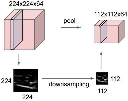
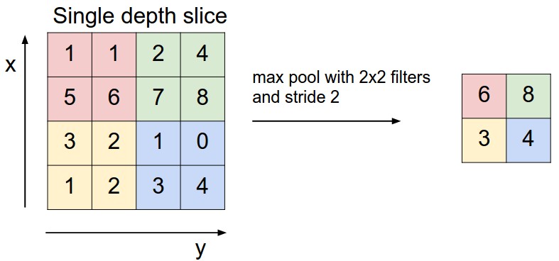
Pooling layer downsamples the volume spatially, independently in each depth slice of the input volume. Left: In this example, the input volume of size [224x224x64] is pooled with filter size 2, stride 2 into output volume of size [112x112x64]. Notice that the volume depth is preserved. Right: The most common downsampling operation is max, giving rise to max pooling, here shown with a stride of 2. That is, each max is taken over 4 numbers (little 2x2 square).

---

Backpropagation.

Recall from the backpropagation chapter that the backward pass for a max(x, y) operation has a simple interpretation as only routing the gradient to the input that had the highest value in the forward pass. Hence, during the forward pass of a pooling layer it is common to keep track of the index of the max activation (sometimes also called the switches) so that gradient routing is efficient during backpropagation.

Getting rid of pooling.

Many people dislike the pooling operation and think that we can get away without it. For example, Striving for Simplicity: The All Convolutional Net proposes to discard the pooling layer in favor of architecture that only consists of repeated CONV layers. To reduce the size of the representation they suggest using larger stride in CONV layer once in a while. Discarding pooling layers has also been found to be important in training good generative models, such as variational autoencoders (VAEs) or generative adversarial networks (GANs). It seems likely that future architectures will feature very few to no pooling layers.

Normalization Layer

Many types of normalization layers have been proposed for use in ConvNet architectures, sometimes with the intentions of implementing inhibition schemes observed in the biological brain. However, these layers have since fallen out of favor because in practice their contribution has been shown to be minimal, if any. For various types of normalizations, see the discussion in Alex Krizhevsky’s cuda-convnet library API.

Fully-connected layer

Neurons in a fully connected layer have full connections to all activations in the previous layer, as seen in regular Neural Networks. Their activations can hence be computed with a matrix multiplication followed by a bias offset. See the Neural Network section of the notes for more information.

Converting FC layers to CONV layers

It is worth noting that the only difference between FC and CONV layers is that the neurons in the CONV layer are connected only to a local region in the input, and that many of the neurons in a CONV volume share parameters. However, the neurons in both layers still compute dot products, so their functional form is identical. Therefore, it turns out that it’s possible to convert between FC and CONV layers:

• For any CONV layer there is an FC layer that implements the same forward function. The weight matrix would be a large matrix that is mostly zero except for at certain blocks (due to local connectivity) where the weights in many of the blocks are equal (due to parameter sharing).

• Conversely, any FC layer can be converted to a CONV layer. For example, an FC layer with $K=4096$ that is looking at some input volume of size $7×7×512$ can be equivalently expressed as a CONV layer with $F=7,P=0,S=1,K=4096$. In other words, we are setting the filter size to be exactly the size of the input volume, and hence the output will simply be $1×1×4096$ since only a single depth column “fits” across the input volume, giving identical result as the initial FC layer.

SUMMARY : 上述 FC layer with $K=4096$ 中的$K$是什么意思？neuron个数？应该是的，可以进行倒推，既然FC layer可以等价的转换为**CONV layer** with $F=7,P=0,S=1,K=4096$，这个**CONV layer**锁执行的操作是非常简单的：它有4096个 filter，每个filter都会和 input volume of size $7×7×512$ 执行dot product，显然这其实就是MLP中的全连接层了，显然，每个filter就相当于MLP中的一个neuron；这个推测在下面的**FC->CONV conversion**中是可以验证的；

SUMMARY : CONV layer with $F=7,P=0,S=1,K=4096$. 中的$K$指的是filter的个数。

FC->CONV conversion.

Of these two conversions, the ability to convert an FC layer to a CONV layer is particularly useful in practice. Consider a ConvNet architecture that takes a 224x224x3 image, and then uses a series of CONV layers and POOL layers to reduce the image to an activations volume of size 7x7x512 (in an AlexNet architecture that we’ll see later, this is done by use of 5 pooling layers that downsample the input spatially by a factor of two each time, making the final spatial size 224/2/2/2/2/2 = 7). From there, an AlexNet uses two FC layers of size 4096 and finally the last FC layers with 1000 neurons that compute the class scores. We can convert each of these three FC layers to CONV layers as described above:

• Replace the first FC layer that looks at [7x7x512] volume with a CONV layer that uses filter size $F=7$, giving output volume [1x1x4096].
• Replace the second FC layer with a CONV layer that uses filter size $F=1$, giving output volume [1x1x4096]
• Replace the last FC layer similarly, with $F=1$, giving final output [1x1x1000]

Each of these conversions could in practice involve manipulating (e.g. reshaping) the weight matrix $W$ in each FC layer into CONV layer filters. It turns out that this conversion allows us to “slide” the original ConvNet very efficiently across many spatial positions in a larger image, in a single forward pass.

For example, if 224x224 image gives a volume of size [7x7x512] - i.e. a reduction by 32, then forwarding an image of size 384x384 through the converted architecture would give the equivalent volume in size [12x12x512], since 384/32 = 12. Following through with the next 3 CONV layers that we just converted from FC layers would now give the final volume of size [6x6x1000], since (12 - 7)/1 + 1 = 6. Note that instead of a single vector of class scores of size [1x1x1000], we’re now getting an entire 6x6 array of class scores across the 384x384 image.

Evaluating the original ConvNet (with FC layers) independently across 224x224 crops of the 384x384 image in strides of 32 pixels gives an identical result to forwarding the converted ConvNet one time.

Naturally, forwarding the converted ConvNet a single time is much more efficient than iterating the original ConvNet over all those 36 locations, since the 36 evaluations share computation. This trick is often used in practice to get better performance, where for example, it is common to resize an image to make it bigger, use a converted ConvNet to evaluate the class scores at many spatial positions and then average the class scores.

Lastly, what if we wanted to efficiently apply the original ConvNet over the image but at a stride smaller than 32 pixels? We could achieve this with multiple forward passes. For example, note that if we wanted to use a stride of 16 pixels we could do so by combining the volumes received by forwarding the converted ConvNet twice: First over the original image and second over the image but with the image shifted spatially by 16 pixels along both width and height.

• An IPython Notebook on Net Surgery shows how to perform the conversion in practice, in code (using Caffe)

ConvNet Architectures

We have seen that Convolutional Networks are commonly made up of only three layer types: CONV, POOL (we assume Max pool unless stated otherwise) and FC (short for fully-connected). We will also explicitly write the RELU activation function as a layer, which applies elementwise non-linearity. In this section we discuss how these are commonly stacked together to form entire ConvNets.

Layer Patterns

The most common form of a ConvNet architecture stacks a few CONV-RELU layers, follows them with POOL layers, and repeats this pattern until the image has been merged spatially to a small size. At some point, it is common to transition to fully-connected layers. The last fully-connected layer holds the output, such as the class scores. In other words, the most common ConvNet architecture follows the pattern:

INPUT -> [[CONV -> RELU]*N -> POOL?]*M -> [FC -> RELU]*K -> FC

where the * indicates repetition, and the POOL? indicates an optional pooling layer. Moreover, N >= 0 (and usually N <= 3), M >= 0, K >= 0 (and usually K < 3). For example, here are some common ConvNet architectures you may see that follow this pattern:

• INPUT -> FC, implements a linear classifier. Here N = M = K = 0.
• INPUT -> CONV -> RELU -> FC
• INPUT -> [CONV -> RELU -> POOL]*2 -> FC -> RELU -> FC. Here we see that there is a single CONV layer between every POOL layer.
• INPUT -> [CONV -> RELU -> CONV -> RELU -> POOL]*3 -> [FC -> RELU]*2 -> FC Here we see two CONV layers stacked before every POOL layer. This is generally a good idea for larger and deeper networks, because multiple stacked CONV layers can develop more complex features of the input volume before the destructive pooling operation.

Additional Resources

Additional resources related to implementation:

• Soumith benchmarks for CONV performance
• ConvNetJS CIFAR-10 demo allows you to play with ConvNet architectures and see the results and computations in real time, in the browser.
• Caffe, one of the popular ConvNet libraries.
• State of the art ResNets in Torch7