Quick sort
wikipedia Quicksort
Quicksort (sometimes called partition-exchange sort) is an efficient sorting algorithm, serving as a systematic method for placing the elements of a random access file or an array in order.
Developed by British computer scientist Tony Hoare in 1959[1] and published in 1961,[2] it is still a commonly used algorithm for sorting.
When implemented well, it can be about two or three times faster than its main competitors, merge sort and heapsort.
Quicksort is a comparison sort, meaning that it can sort items of any type for which a "less-than" relation (formally, a total order) is defined.
Efficient implementations of Quicksort are not a stable sort, meaning that the relative order of equal sort items is not preserved.
Quicksort can operate in-place on an array, requiring small additional amounts of memory to perform the sorting. It is very similar to selection sort, except that it does not always choose worst-case partition.
Mathematical analysis of quicksort shows that, on average, the algorithm takes O(n log n) comparisons to sort n items. In the worst case, it makes O(n^2) comparisons, though this behavior is rare.
Algorithm
Quicksort is a divide and conquer algorithm. Quicksort first divides a large array into two smaller sub-arrays: the low elements and the high elements. Quicksort can then recursively sort the sub-arrays. The steps are:
1、Pick an element, called a pivot(基准), from the array.
2、Partitioning: reorder the array so that all elements with values less than the pivot come before the pivot, while all elements with values greater than the pivot come after it (equal values can go either way). After this partitioning, the pivot is in its final position. This is called the partition operation.
3、Recursively apply the above steps to the sub-array of elements with smaller values and separately to the sub-array of elements with greater values.
The base case of the recursion is arrays of size zero or one, which are in order by definition, so they never need to be sorted.
The pivot selection and partitioning steps can be done in several different ways; the choice of specific implementation schemes greatly affects the algorithm's performance.
Implementation issues
Parallelization
Quicksort's divide-and-conquer formulation makes it amenable to parallelization using task parallelism. The partitioning step is accomplished through the use of a parallel prefix sum algorithm to compute an index for each array element in its section of the partitioned array.[23][24] Given an array of size n, the partitioning step performs O(n) work in O(log n) time and requires O(n) additional scratch space. After the array has been partitioned, the two partitions can be sorted recursively in parallel. Assuming an ideal choice of pivots, parallel quicksort sorts an array of size n in O(n log n) work in O(log² n) time using O(n) additional space.
Formal analysis
NOTE:
一、以下分析是使用quicksort中所执行的比较的次数来作为复杂性计算的单位的;
其实quicksort的比较都是发生在
partition函数中;二、为了便于分析,可以以quick sort一个长度为5的array为例来进行说明

Worst-case analysis
The most unbalanced partition occurs when one of the sublists returned by the partitioning routine is of size n − 1.[27] This may occur if the pivot happens to be the smallest or largest element in the list, or in some implementations (e.g., the Lomuto partition scheme as described above) when all the elements are equal.
If this happens repeatedly in every partition, then each recursive call processes a list of size one less than the previous list. Consequently, we can make n − 1 nested calls before we reach a list of size 1. This means that the call tree is a linear chain of n − 1 nested calls. The i*th call does *O(n − i) work to do the partition, and $ \textstyle \sum _{i=0}{n}(n-i)=O(n^{2}) $, so in that case Quicksort takes O(*n*²) time.
NOTE:
一、其实这种情况本质上是BST退化为了linked list,此时树的高度为n。
第0次调用quicksort需要进行n此比较,第1次调用quicksort需要进行n-1次比较,依次类推,所以总的耗费为n此调用之和;所以就是$ \textstyle \sum _{i=0}{n}(n-i)=O(n^{2}) $;
这种情况其实就是Bubble sort,算法复杂度就是O(n^{2})
二、以quick sort一个长度为5的array为例来进行说明
Best-case analysis
In the most balanced case, each time we perform a partition we divide the list into two nearly equal pieces. This means each recursive call processes a list of half the size. Consequently, we can make only log_2{n} nested calls before we reach a list of size 1. This means that the depth of the call tree is log_2{n}. But no two calls at the same level of the call tree process the same part of the original list; thus, each level of calls needs only O(n) time all together (each call has some constant overhead, but since there are only O(n) calls at each level, this is subsumed in the O(n) factor). The result is that the algorithm uses only O(n log n) time.
NOTE:
一、上述分析是能够帮助我们理解quick sort的computation complexity的,它是非常简单易懂的
二、上述complexity analysis,使用到了 binary search 的 computation complexity analysis:
在均衡的情况下,树的高度为logn,每层的比较次数为n,因此总的computation complexity为: O(n log n)
三、best-case其实是非常类似于balanced binary search tree的;
Average-case analysis
NOTE: 下面设计了很多的数学推导,比较难以理解,我们重点关注"Using a binary search tree"
To sort an array of n distinct elements, quicksort takes O(n log n) time in expectation, averaged over all n! permutations of n elements with equal probability. We list here three common proofs to this claim providing different insights into quicksort's workings.
Using percentiles百分位数值
Using recurrences
Using a binary search tree
NOTE:
一、quick sort隐式地构造了一颗BST
To each execution of quicksort corresponds the following binary search tree (BST):
the initial pivot is the root node;
the pivot of the left half is the root of the left subtree,
the pivot of the right half is the root of the right subtree, and so on.
The number of comparisons of the execution of quicksort equals the number of comparisons during the construction of the BST by a sequence of insertions. So, the average number of comparisons for randomized quicksort equals the average cost of constructing a BST when the values inserted $ (x_{1},x_{2},\ldots ,x_{n}) $ form a random permutation.
Consider a BST created by insertion of a sequence $ (x_{1},x_{2},\ldots ,x_{n}) $ of values forming a random permutation. Let C denote the cost of creation of the BST. We have $ C=\sum {i}\sum *{j<i}c*{i,j} $, where $ c{i,j} $ is an binary random variable expressing whether during the insertion of $ x_{i} $ there was a comparison to $ x_{j} $.
By linearity of expectation, the expected value $ \operatorname {E} [C] $ of C is $ \operatorname {E} [C]=\sum _{i}\sum {j<i}\Pr(c{i,j}) $.
Fix i and j<i. The values $ {x_{1},x_{2},\ldots ,x_{j}} $, once sorted, define j+1 intervals. The core structural observation is that $ x_{i} $ is compared to $ x_{j} $ in the algorithm if and only if $ x_{i} $ falls inside one of the two intervals adjacent to $ x_{j} $.
Observe that since $ (x_{1},x_{2},\ldots ,x_{n}) $ is a random permutation, $ (x_{1},x_{2},\ldots ,x_{j},x_{i}) $ is also a random permutation, so the probability that $ x_{i} $ is adjacent to $ x_{j} $ is exactly $ {\frac {2}{j+1}} $.
We end with a short calculation:
$ \operatorname {E} [C]=\sum _{i}\sum _{j<i}{\frac {2}{j+1}}=O\left(\sum _{i}\log i\right)=O(n\log n). $
Relation to other algorithms
Quicksort is a space-optimized version of the binary tree sort. Instead of inserting items sequentially into an explicit tree, quicksort organizes them concurrently into a tree that is implied by the recursive calls. The algorithms make exactly the same comparisons, but in a different order.
NOTE:
一、quick sort隐式地构造了一颗BST
An often desirable property of a sorting algorithm is stability – that is the order of elements that compare equal is not changed, allowing controlling order of multikey tables (e.g. directory or folder listings) in a natural way. This property is hard to maintain for in situ(原位) (or in place) quicksort (that uses only constant additional space for pointers and buffers, and O(log n) additional space for the management of explicit or implicit recursion). For variant quicksorts involving extra memory due to representations using pointers (e.g. lists or trees) or files (effectively lists), it is trivial to maintain stability. The more complex, or disk-bound, data structures tend to increase time cost, in general making increasing use of virtual memory or disk.
The most direct competitor of quicksort is heapsort. Heapsort's running time is O(n log n), but heapsort's average running time is usually considered slower than in-place quicksort. This result is debatable; some publications indicate the opposite.[28][29] Introsort is a variant of quicksort that switches to heapsort when a bad case is detected to avoid quicksort's worst-case running time.
Quicksort also competes with merge sort, another O(n log n) sorting algorithm. Mergesort is a stable sort, unlike standard in-place quicksort and heapsort, and can be easily adapted to operate on linked lists and very large lists stored on slow-to-access media such as disk storage or network-attached storage. Although quicksort can be implemented as a stable sort using linked lists, it will often suffer from poor pivot choices without random access. The main disadvantage of mergesort is that, when operating on arrays, efficient implementations require O(n) auxiliary space, whereas the variant of quicksort with in-place partitioning and tail recursion uses only O(log n) space. (When operating on linked lists, mergesort only requires a small, constant amount of auxiliary storage.)
Bucket sort with two buckets is very similar to quicksort; the pivot in this case is effectively the value in the middle of the value range, which does well on average for uniformly distributed inputs.
Implementation
计算机算法设计与分析


完整程序
#include <cstdio>
#include <iostream>
#include <algorithm>
/**
* @param start 数组起始下标
* @param end 数组终止下标
**/
template<typename T>
void QuickSort(T a[], int start, int end);
template<typename T>
int Partition(T a[], int start, int end);
template<typename T>
void Swap(T& a, T& b)
{
T tmp = a;
a = b;
b = tmp;
}
/*Displays the array, passed to this method*/
template<typename T>
void display(T arr[], int n);
int main()
{
int n;
std::cout << "Enter size of array:\n";
std::cin >> n; // E.g. 8
std::cout << "Enter the elements of the array\n";
int i;
int *arr = new int[n];
for (i = 0; i < n; i++)
{
std::cin >> arr[i];
}
std::cout << "Original array: ";
display(arr, n); // Original array : 10 11 9 8 4 7 3 8
QuickSort(arr, 0, n - 1);
std::cout << "Sorted array: ";
display(arr, n); // Sorted array : 3 4 7 8 8 9 10 11
getchar();
return 0;
}
/**
* @param start 数组起始下标
* @param end 数组终止下标
**/
template<typename T>
void QuickSort(T a[], int start, int end)
{
if (start < end)
{
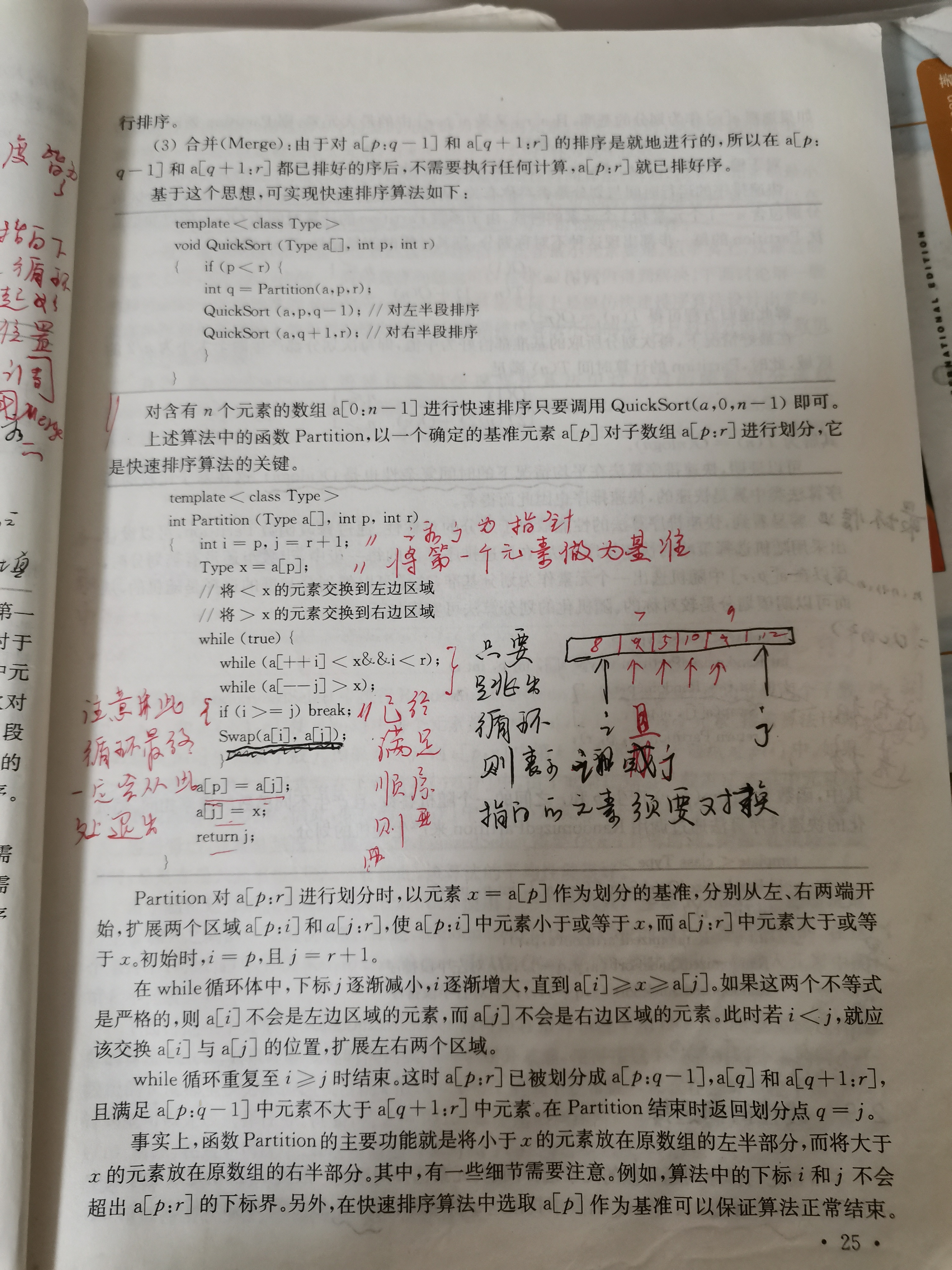
int p = Partition(a, start, end); // pivot index
QuickSort(a, start, p - 1); // 对左半段排序
QuickSort(a, p + 1, end); // 对右半段排序
}
}
template<typename T>
int Partition(T a[], int start, int end)
{
int i = start, j = end + 1;
T pivot = a[start];
while (true)
{
while (a[++i] < pivot and i < end)
;
while (a[--j] > pivot)
;
if (i >= j)
break;
std::swap(a[i], a[j]); // 使用标准库的swap函数
}
a[start] = a[j];
a[j] = pivot;
return j;
}
/*Displays the array, passed to this method*/
template<typename T>
void display(T arr[], int n)
{
int i;
for (i = 0; i < n; i++)
{
std::cout << arr[i] << " ";
}
std::cout << "\n";
}
测试用例:[5, 4, 3, 2, 1]
使用上述算法对[5, 4, 3, 2, 1]进行排序:while(a[++i]<x and i<end);退出时,i的值为end即4;while(a[--j]>x);退出时,j的值为4。
测试用例:[10, 11, 9, 8, 4, 7, 3, 8]
randomized_partition 避免退化
当原数组本身是有序的时候,如果每次都选择第一个元素作为pivot,那么将导致quick sort退化,下面是源自: https://leetcode-cn.com/submissions/detail/194476777/testcase/
[1,2,3,4,5,6,7,8,9,10,11,12,13,14,15,16,17,18,19,20,21,22,23,24,25,26,27,28,29,30,31,32,33,34,35,36,37,38,39,40,41,42,43,44,45,46,47,48,49,50,51,52, ......50000]
这种情况下是会超时的。
class Solution {
    int partition(vector<int>& nums, int l, int r) {
        int pivot = nums[r];
        int i = l - 1;
        for (int j = l; j <= r - 1; ++j) {
            if (nums[j] <= pivot) {
                i = i + 1;
                swap(nums[i], nums[j]);
            }
        }
        swap(nums[i + 1], nums[r]);
        return i + 1;
    }
    int randomized_partition(vector<int>& nums, int l, int r) {
        int i = rand() % (r - l + 1) + l; // 随机选一个作为我们的主元
        swap(nums[r], nums[i]);
        return partition(nums, l, r);
    }
    void randomized_quicksort(vector<int>& nums, int l, int r) {
        if (l < r) {
            int pos = randomized_partition(nums, l, r);
            randomized_quicksort(nums, l, pos - 1);
            randomized_quicksort(nums, pos + 1, r);
        }
    }
public:
    vector<int> sortArray(vector<int>& nums) {
        srand((unsigned)time(NULL));
        randomized_quicksort(nums, 0, (int)nums.size() - 1);
        return nums;
    }
};
hackerearth Quick Sort
讲解地非常不错。
partition
int partition ( int A[],int start ,int end) {
    int i = start + 1;
    int piv = A[start] ;            //make the first element as pivot element.
    for(int j =start + 1; j <= end ; j++ )  {
    /*rearrange the array by putting elements which are less than pivot
       on one side and which are greater that on other. */

          if ( A[ j ] < piv) {
                 swap (A[ i ],A [ j ]);
            i += 1;
        }
   }
   swap ( A[ start ] ,A[ i-1 ] ) ;  //put the pivot element in its proper place.
   return i-1;                      //return the position of the pivot
}
i是用于定界的。
函数的返回值是分割位置。
使用fast、slow pointer来解释partition
/**
 * @brief
 * 我们让慢指针`slow`走在后面,快指针`fast`走在前面探路,找到一个不重复的元素就告诉`slow`并让`slow`前进一步。
 * 这样当`fast`指针遍历完整个数组`nums`后,**`nums[0..slow]`就是不重复元素**。
 * slow指向的是右侧大于pivot的第一个元素,显然,它记录的是右半段的左侧边界;
 * pivot的过程其实是不断地将右侧区间中的不属于它的元素、即属于左侧区间的元素拿到左侧区间,
 * 那么它如何实现呢?其实方法非常简答: 让出一个位置的元素给左侧区间来存放刚刚找到的这个元素
 * 这个函数,被调用的前提是 start > end,因此最少的情况: end = start + 1
 * 刚开始的时候,fast 和 slow的值是相等的,这是必须的,因为可能只有start、end两个元素,如果让end指向start后的一个元素,则存在如下可能性:
 * 1、数组越界
 * 2、无法进入到后面的交换环节,即使只有两个元素,这也是需要进行交换的
 * @param A
 * @param start
 * @param end
 * @return
 */
int partition(int A[], int start, int end)
{
    int slow = start + 1;
    int piv = A[start];            //make the first element as pivot element.
    for (int fast = start + 1; fast <= end; fast++)
    {
        /*rearrange the array by putting elements which are less than pivot
         on one side and which are greater that on other. */
        if (A[fast] < piv)
        {
            swap(A[slow], A[fast]);
            slow += 1;
        }
    }
    swap(A[start], A[slow - 1]);  //put the pivot element in its proper place.
    return slow - 1;                      //return the position of the pivot
}
完整程序
Now, let us see the recursive function Quick_sort :
void quick_sort ( int A[ ] ,int start , int end ) {
   if( start < end ) {
        //stores the position of pivot element
         int piv_pos = partition (A,start , end ) ;
         quick_sort (A,start , piv_pos -1);    //sorts the left side of pivot.
         quick_sort ( A,piv_pos +1 , end) ; //sorts the right side of pivot.
   }
}
完整程序如下:
#include <stdio.h>
#include <stdlib.h>

/*Displays the array, passed to this method*/
void display(int arr[], int n)
{

    int i;
    for (i = 0; i < n; i++)
    {
        printf("%d ", arr[i]);
    }

    printf("\n");
}

/*Swap function to swap two values*/
void swap(int *first, int *second)
{

    int temp = *first;
    *first = *second;
    *second = temp;
}


int partition ( int A[],int start ,int end) {
    int i = start + 1;
    int piv = A[start] ;            //make the first element as pivot element.
    for(int j =start + 1; j <= end ; j++ )  {
    /*rearrange the array by putting elements which are less than pivot
       on one side and which are greater that on other. */

          if ( A[ j ] < piv) {
                 swap (A[ i ],A [ j ]);
            i += 1;
        }
   }
   swap ( A[ start ] ,A[ i-1 ] ) ;  //put the pivot element in its proper place.
   return i-1;                      //return the position of the pivot
}

/*This is where the sorting of the array takes place
    arr[] --- Array to be sorted
    lower --- Starting index
    upper --- Ending index
*/
void quickSort(int arr[], int lower, int upper)
{

    if (upper > lower)
    {

        // partitioning index is returned by the partition method , partition element is at its correct poition

        int partitionIndex = partition(arr, lower, upper);

        // Sorting elements before and after the partition index
        quickSort(arr, lower, partitionIndex - 1);
        quickSort(arr, partitionIndex + 1, upper);
    }
}

int main()
{

    int n;
    printf("Enter size of array:\n");
    scanf("%d", &n); // E.g. 8

    printf("Enter the elements of the array\n");
    int i;
    int *arr = (int *)malloc(sizeof(int) * n);
    for (i = 0; i < n; i++)
    {
        scanf("%d", &arr[i]);
    }

    printf("Original array: ");
    display(arr, n); // Original array : 10 11 9 8 4 7 3 8

    quickSort(arr, 0, n - 1);

    printf("Sorted array: ");
    display(arr, n); // Sorted array : 3 4 7 8 8 9 10 11
    getchar();
    return 0;
}
对比两种实现方式
上述两种实现方式,其实都使用了double pointer:
1、“计算机算法设计与分析”中的实现的思路是:由两端向中间扩展
2、“hackerearth Quick Sort”中的实现方式的思路是:自左向右进行扩展、fast-slow double pointer。
分三段,只需要两个boundary,分别对应i和j。
TODO
developer.51cto 坐在马桶上看算法:快速排序